Looking at Pictures topological analysis of patterns
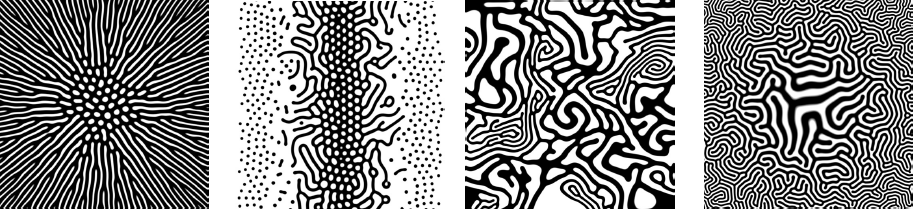 Image from Karl Sims.
Image from Karl Sims.
Image from Karl Sims.
Patterns exist on every scale; from a spiral galaxy down to the dendrites of a snowflake. There is no unifying theory to describe pattern formation but there are canonical ways to analyze.
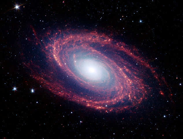
M81 galaxy (NASA).
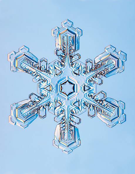
Hexagonal snowflake dendrite (Kenneth Libbrecht).
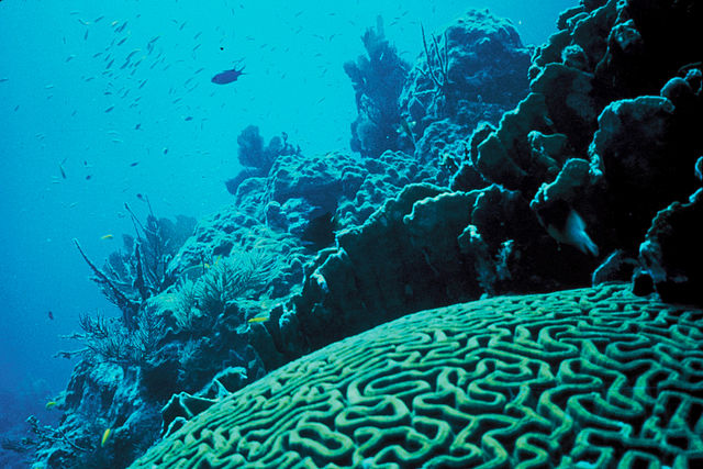
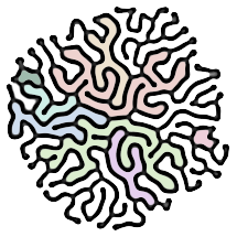
Coral displays interesting pattern (U.S. Fish and Wildlife).
Rayleigh-Benard convection (Kurtuldu 2010).
Belousov–Zhabotinsky reaction (Stephen Morris, UofT).
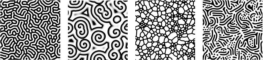
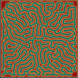
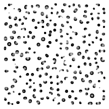
Gray-Scott system (Karl Sims).
More data is great, but as the complexity of a system increases it becomes more difficult to extract relevant information.
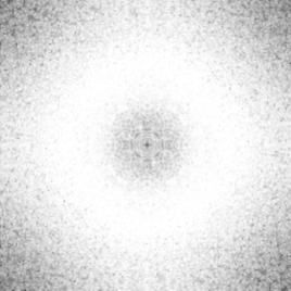
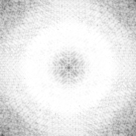
The Fourier-Transform is a common method for pattern analysis, but for a complex pattern, it is difficult to draw conclusions from these methods → need new paradigms
Pattern alpha α
Fast Fourier transform of alpha α
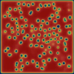
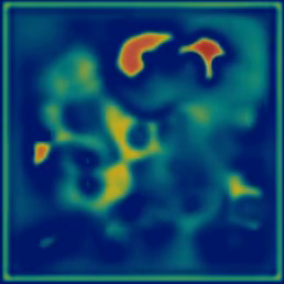
Pattern kappa κ
Fast Fourier tranfsorm of kappa κ
Reaction-diffusion (RD) systems determine how concentrations of substances change in space driven by two processes: chemical reaction and spatial diffusion. What makes them interesting is the wide variety of patterns they form and how many of those patterns resemble patterns of nature (e.g. spirals, stripes, and spots). In 1952, Alan Turing suggested that RD systems of morphogens may explain the presence of spots or stripes on an organism like a cheetah or zebra (Turing 1952). Turns out he was wrong but Turing laid the framework by which patterns form from minor perturbations of otherwise homogenous systems. Since then these types of systems have been studied extensively.
Characterizes chemical interaction
U + 2V → 3V,
V → P.
Modeled by the following PDEs. $$ \frac{\partial u}{\partial t} = d_u \nabla^2 u - uv^2 + F(1-u) \\ \frac{\partial v}{\partial t} = d_v \nabla^2 v + uv^2 - (F
+k)v $$
For different (F, k), Pearson (1993) identified 14 different pattern types (see figure). The region near the bifurcation lines is the least stable and thus gives the most interesting patterns.
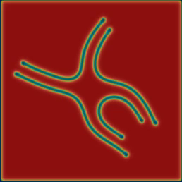
alpha exhibits spatio-temporal chaos. wavelets and "fledgeling-spirals" collide and annihilate upon hitting another.
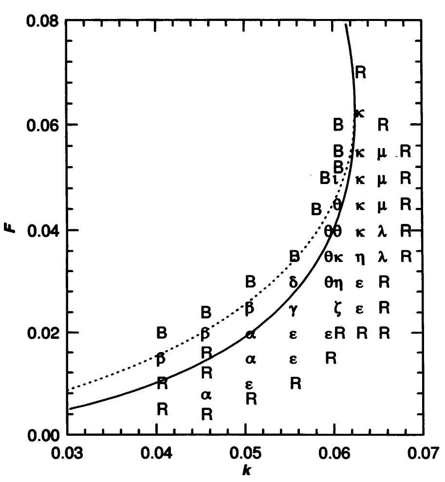
A plot of (F,k) parameter space (Pearson 1993).
Homology is a method of extracting algebraic information from a topological space. This has the benefit of being extremely low-level by focusing on the geometric structures. We are primarily concerned with the Betti Numbers, or βi
β0 = 1
β1 = 1
β0 = 2
β1 = 1
β0 = 1
β1 = 0
β0 = 1
β1 = 1
Homology of alpha α
β0 = 223
β1 = 1
Homology of kappa κ
β0 = 1
β1 = 9
Choose a pattern below to see how the Betti numbers of a pattern change over time. The pairs {β0,β1}i can be said to represent a 'state' of the system.
alpha exhibits spatio-temporal chaos. wavelets and "fledgeling-spirals" collide and annihilate upon hitting another.
β0 | β1
Time steps
Given a state {β0,β1}i, we can define
$$ S = - \sum_{i=1}^{N} P_i \log{P_i}. $$ S gives a measure of complexity of the system. Intuitively, it represents how easily we can predict the next state.
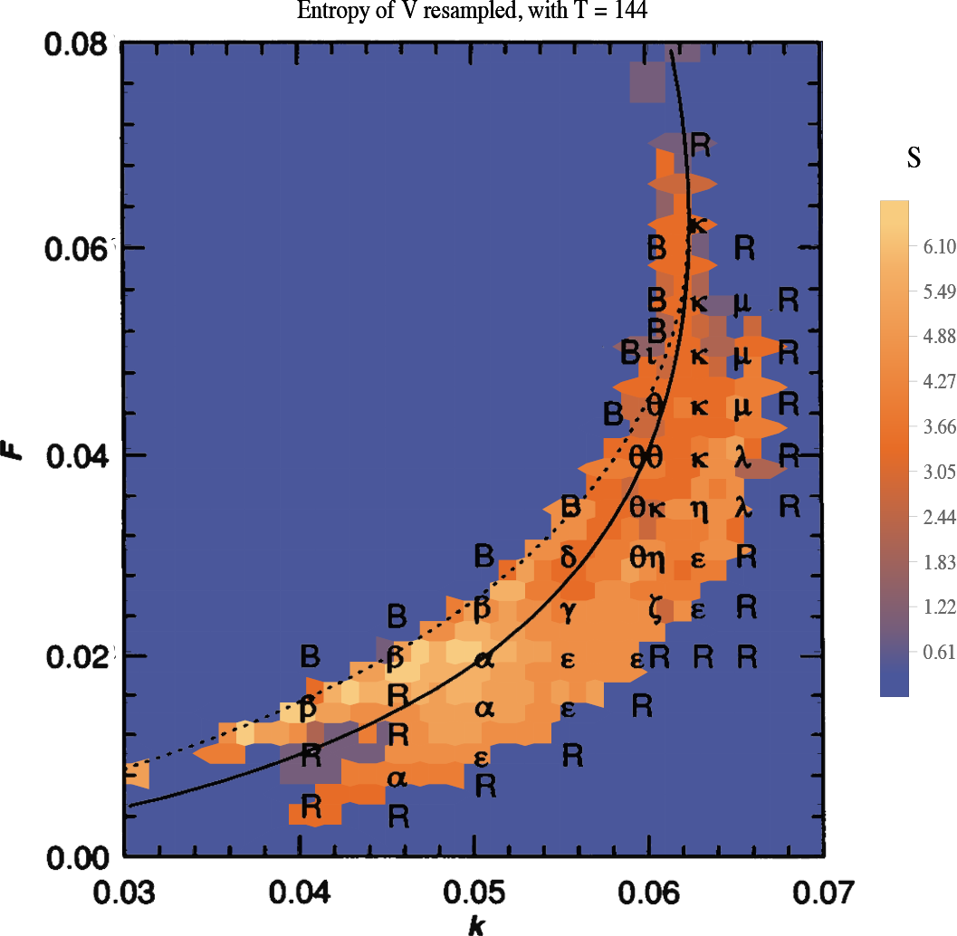
The plot shows the entropy S over (F,k) parameter space.
How does the complexity information encoded in entropy relate to Pearson's data? Does it uncover more about the parameter space?
Open questions:
Homology is low-level analysis, but low-level geometric methods are the building blocks for higher levels of image analysis (e.g. fingerprint scanning, character recognization etc.).